Example: XGBoost power loss

This examples shows you how to load the trained XGBoost model and use it.

import os
from pathlib import Path

project_root = Path.cwd().parents[1]
os.chdir(project_root)   # now cwd is .../pvcracks

from pvcracks.powerloss.powerloss_functions import load_xgb_models, predict_power_and_voc
import numpy as np
import pandas as pd

Calculate delta Pmpp from fitted IV cell curves

Cell9Master = pd.read_csv('docs/data/ELdata_module_209_VAE_analysis.csv', index_col=0)

# grab each Module’s Init‐stage Pmp
init = (
    Cell9Master[Cell9Master['Deg']=='Init']
    .set_index('Module')['Pmp']
    # init is now a Series: index=Module, value=Pmp_at_Init
)

# Calcuate differenc in %
Cell9Master['deltaPmp'] = 100*(Cell9Master['Pmp'] - Cell9Master['Module'].map(init))/Cell9Master['Module'].map(init)

#Filter out specific cells we know have cracks
cracked = [
    ('209_A2','Deg1'),
    ('209_A1','Deg1'),
    ('209_A3','Deg2'),
    ('209_A1','Deg2'),
    ('209_C3','Deg2'),
    ('209_B2','Deg2'),
    ('209_B3','Deg2'),
]

# 2) build a boolean mask which is True only for those pairs
mask = Cell9Master[['Module','Deg']].apply(tuple,axis=1).isin(cracked)

# 3) slice to keep only the cracked cells
Cell9Degs = Cell9Master[mask].copy()

Cell9Degs

	ELPath	Module	Deg	Rs	Rsh	I	Is	N	Pmp	Vmp	Imp	lat_vec	klabel	deltaPmp
11	/docs/data/EL/209_A2/Deg1/209_A2_0005_2021_04_...	209_A2	Deg1	0.008996	1295.750000	8.228613	9.005018e-08	1.317542	3.534448	0.465455	7.593540	[ 5.0129116e-02 1.5392177e+00 1.2010708e+00 ...	4	-0.254354
12	/docs/data/EL/209_A1/Deg1/209_A1_0005_2021_04_...	209_A1	Deg1	0.010386	1.000000	8.184377	1.006196e-05	1.778587	3.051399	0.446061	6.840773	[ 0.1527828 0.6933546 0.61783403 -1.311733...	1	-13.414670
18	/docs/data/EL/209_A3/Deg2/209_A3_0005_2021_04_...	209_A3	Deg2	0.008634	8.986411	8.233849	6.987570e-06	1.730266	3.349300	0.458990	7.297111	[ 1.6261781e+00 -1.3577162e-01 3.6160046e-01 ...	4	-6.030860
21	/docs/data/EL/209_A1/Deg2/209_A1_0005_2021_04_...	209_A1	Deg2	0.012567	0.835178	7.588188	3.762260e-05	1.997049	2.678277	0.433131	6.183523	[-1.2965436 0.14127842 0.39876893 -0.320378...	1	-24.002233
23	/docs/data/EL/209_C3/Deg2/209_C3_0005_2021_04_...	209_C3	Deg2	0.009595	88.786965	8.160221	1.795159e-06	1.573030	3.347141	0.452525	7.396585	[-4.2912847e-01 2.1230426e+00 8.3105731e-01 ...	3	-3.268041
25	/docs/data/EL/209_B2/Deg2/209_B2_0005_2021_04_...	209_B2	Deg2	0.009456	529.959186	8.231207	3.558481e-06	1.644547	3.346776	0.452525	7.395777	[-0.2521562 0.70483327 1.0419804 -1.359632...	1	-4.311519
26	/docs/data/EL/209_B3/Deg2/209_B3_0005_2021_04_...	209_B3	Deg2	0.010031	97.047204	8.309195	1.610765e-06	1.567835	3.399534	0.452525	7.512363	[-1.8619239 1.6475563 1.0302961 -1.493011...	1	-4.495282

Load latent vectors:

We show in the EL variational autoencoder (VAE) example “Rapid EL processing” how to obtain these.

#reformat latent vectors to np.array[np.array[],...]
def parse_whitespace_vec(s):
    # strip off the brackets, then split on any whitespace (incl newlines),
    # then convert each token to float
    nums = s.strip('[]').split()
    return [float(x) for x in nums]

# apply parsing
parsed = Cell9Degs['lat_vec'].apply(parse_whitespace_vec)

# 2) stack into a numpy array of dtype object
lat_vectors = np.array(parsed.tolist(), dtype=object)

Load xgboost models:

pmpp_model, voc_model = load_xgb_models(
        pmpp_model_path="pvcracks/powerloss/xgb_model_pmpp_diff_percent_3CH.pkl",
        voc_model_path="pvcracks/powerloss/xgb_model_Voc_diff_percent_3CH.pkl"
    )

Predict delta Pmpp in %

df_predictions = predict_power_and_voc(lat_vectors, pmpp_model, voc_model)

#power loss predictions added to cell info dataframe
Cell9Degs.loc[:, 'power_loss_%'] = df_predictions['power_loss_%'].values

Cell9Degs[['Module', 'Deg', 'deltaPmp', 'power_loss_%']]

	Module	Deg	deltaPmp	power_loss_%
11	209_A2	Deg1	-0.254354	-13.171658
12	209_A1	Deg1	-13.414670	-12.675356
18	209_A3	Deg2	-6.030860	-15.003642
21	209_A1	Deg2	-24.002233	-10.363716
23	209_C3	Deg2	-3.268041	-7.291249
25	209_B2	Deg2	-4.311519	-18.673622
26	209_B3	Deg2	-4.495282	-15.299884

#Compare IV fit results vs XGboost
import matplotlib.pyplot as plt

x = Cell9Degs['deltaPmp']
y = Cell9Degs['power_loss_%']

# compute correlation
r = x.corr(y)

plt.figure(figsize=(6,4))
plt.scatter(x, y, alpha=0.7)
mn = min(x.min(), y.min())
mx = max(x.max(), y.max())
plt.plot([mn,mx], [mn,mx], 'r--', label='y = x')
plt.text(x.min()-0.9, 0, f"Pearson r = {r:.3f}", fontsize=10, verticalalignment='top',
        bbox=dict(boxstyle='round', facecolor='white', alpha=0.7))
plt.xlabel('Cell delta Pmp from IV curves (%)')
plt.ylabel('Power Loss from latent vectors and XGboost (%)')
plt.title('IV curve delta Pmpp vs. XGboost power loss %')
plt.legend()
plt.grid(True)
plt.tight_layout()
plt.show()

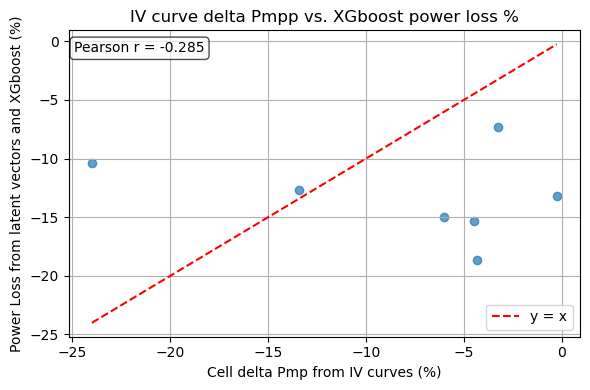
The current results show a low pearson score (<0.3). This is due to our limited amount of EL/IV pairs that we could use to train the XGboost model, 77 pairs. In the powerloss subpackage there is a jupyter notebook going through the steps how the xgboost model is trained. This could be done with more data when made avaialable.